

Confidence Interval to Z Score

You've been handed a confidence interval in a report, and the number you need isn't printed anywhere: the critical z score. The good news is that you can work backward from the interval, as long as you also know the population standard deviation and sample size.
The conversion comes down to a simple idea: the interval's half-width is the margin of error, and the z score tells you how many standard errors make up that margin. Once you see how those pieces fit, the formula is much less intimidating.
What a Confidence Interval and a Z Score Represent
A confidence interval gives a range around a sample estimate rather than a single exact number. Its midpoint is the point estimate, often a sample mean, and the distance from that midpoint to either endpoint is the margin of error. The wider that distance, the more uncertainty the interval admits about where the true population value sits.
For a population mean with a known population standard deviation, the interval looks like this:
[ \bar{x} \pm z_{\alpha/2}\left(\frac{\sigma}{\sqrt{n}}\right) ]
Each symbol earns its place. (\bar{x}) is the sample mean, (\sigma) is the population standard deviation, and (n) is the sample size. The expression (\sigma/\sqrt{n}) is the standard error, which measures how much sample means wiggle around the population mean from one sample to the next. The critical z score, (z_{\alpha/2}), is the multiplier that stretches one standard error out to the full margin of error. OpenStax walks through this formula and each of its components.
The confidence level decides how large that multiplier gets. On the standard normal curve, the confidence level is the shaded central area, with the leftover probability split between two matching tails. For a 95% confidence interval, 5% of the curve's area falls outside the center, and the critical z value of about 1.96 marks where the central region ends and each tail begins. Readers revising normal-curve areas can find practice material in these A-Level statistics resources.
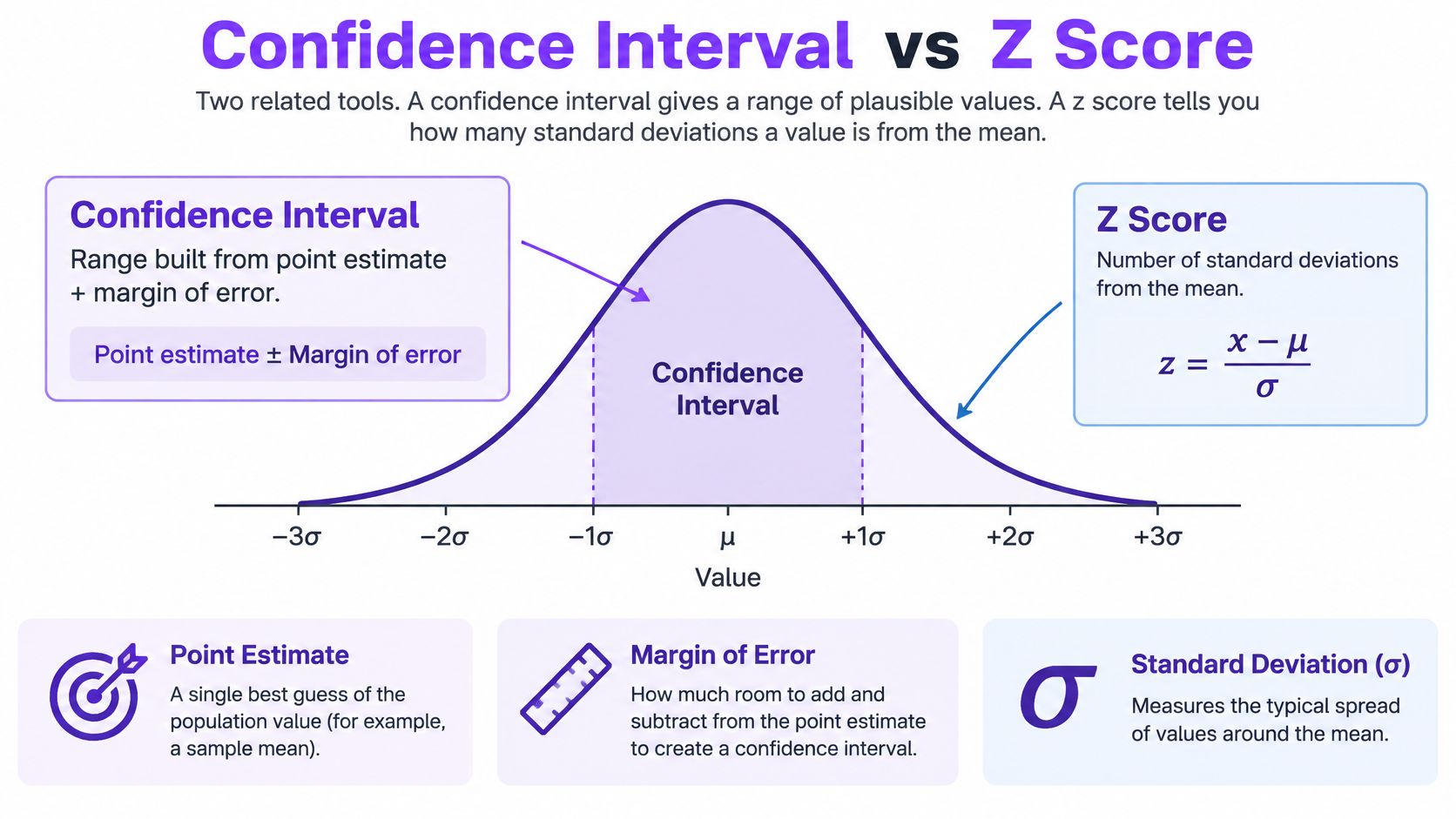
The formula runs in both directions, which is the key to the whole conversion. Going from z to interval, you multiply the critical value by the standard error and add the result to the sample mean. Going from interval to z, you shrink the margin of error back down into standard-error units and recover the multiplier that built it. One caution applies throughout: the z-based method leans on knowing (\sigma). When the population standard deviation is unknown and the sample is small, the normal curve understates the uncertainty, and a different multiplier takes over. The word "confidence" also shows up beyond traditional statistics, where machine-learning confidence scores describe something closer to a model's self-rated certainty than a statistical interval.
Rearranging the Margin of Error to Isolate Z
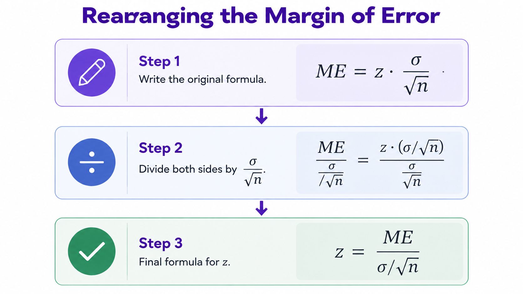
Start with the margin-of-error relationship:
[ ME = z\left(\frac{\sigma}{\sqrt{n}}\right) ]
The term in parentheses is the standard error. In plain language, the equation says that the margin of error equals the number of standard errors represented by the z score, multiplied by the size of one standard error.
To isolate (z), divide both sides by the standard error:
[ \frac{ME}{\sigma/\sqrt{n}}
\frac{z(\sigma/\sqrt{n})}{\sigma/\sqrt{n}} ]
The standard-error terms on the right cancel, leaving:
[ z = \frac{ME}{\sigma/\sqrt{n}} ]
That's the confidence interval to z score conversion. It's the margin of error divided by the standard error.
To get the margin of error from a printed interval, subtract the lower endpoint from the upper endpoint, then divide the full width by two. If the report gives the margin of error directly, use that instead.
Watch the width: The margin of error is the half-width, not the full distance from the lower endpoint to the upper endpoint.
For example, if an interval runs from (L) to (U), its margin of error is ((U-L)/2). Keep that distinction clear before dividing by the standard error. The same relationship also works in reverse: multiply a known z score by the standard error to get the margin of error, then add and subtract it from the estimate to form an interval.
For a visual walkthrough of the algebra, use the video below.
A Worked Example From Interval to Z Score
Take a reported interval for average delivery time: 97.06 to 102.94, with sample mean 100, known population standard deviation 15, and sample size 100. As noted earlier, these values come from the standard textbook setup for a mean with known sigma.
Read the interval as an estimate plus or minus a margin. The midpoint is 100, and each endpoint sits 2.94 away, so the margin of error is 2.94. The same value comes from ((102.94-97.06)/2 = 5.88/2).
That margin is the distance from the center to one edge. The z score asks how many standard errors fit into that distance.
Calculate the standard error first:
[ \frac{\sigma}{\sqrt{n}}
\frac{15}{\sqrt{100}}
1.5 ]
Then divide the margin by that standard error:
[ z = \frac{2.94}{1.5} = 1.96 ]
A result of 1.96 matches the familiar two-sided 95% critical value, so the interval's width lines up with the stated confidence level under a known-sigma normal model.
The mistake that doubles z
The full endpoint-to-endpoint distance is 5.88. Feed that into the formula and z becomes 3.92, which would imply much narrower tails than the report used. Use only one side of the interval.
To run your own check, find (ME), compute (\sigma/\sqrt{n}), divide, then compare with the critical value implied by the confidence level. If your z disagrees, revisit the assumptions before the algebra: a different sigma, a one-sided interval, or a small-sample t method can all change the expected cutoff.
Quick Reference for the Most Common Confidence Levels
If you already know the confidence level, you can usually look up the corresponding critical z score instead of calculating it from an interval. The table below gives the two-sided values available in NIST's reference table. NIST lists the critical z factors for these confidence levels.
| Confidence level | Tail probability (each side) | Two-sided z |
|---|---|---|
| 90% | 5% | 1.645 |
| 95% | 2.5% | 1.960 |
| 99% | 0.5% | 2.575 |
The tail probability is the amount of probability left outside the central interval, divided equally between its two tails. For instance, at 95% confidence, 5% remains outside the interval, so each tail contains 2.5%. The z value marks the cutoff between a tail and the central area.
Two-sided is the important part. These values describe intervals with coverage on both sides of the estimate. A one-sided question places the remaining probability in one tail instead, so its critical value isn't interchangeable with the two-sided value. If a report doesn't clearly say whether the interval is one-sided or two-sided, check its methods before choosing a z score.
Use the table as a lookup, not as a substitute for checking assumptions. It applies when the interval uses the standard normal distribution. Students preparing for statistics exams can also explore Tutorbase's test prep solution for structured study support.
How Interval Width, Sample Size, and Sigma Interact
When you calculate (z=ME/(\sigma/\sqrt{n})), each part of the equation affects the result. The margin of error is in the numerator; the standard error is in the denominator. A wider interval means a larger margin of error, while a larger standard error makes the back-calculated z smaller, assuming the other quantities stay the same.
Consider how each input works when the others are held constant:
- Wider interval: A larger half-width produces a larger calculated z.
- Larger known standard deviation: A larger (\sigma) increases the standard error, so the calculated z is smaller for the same interval width and sample size.
- Larger sample size: A larger (n) reduces the standard error, so the calculated z is larger for the same interval width and known standard deviation.
That last point can feel counterintuitive. If the confidence level stays fixed, increasing the sample size usually makes the interval narrower. But if you hold the interval width fixed and increase the sample size, the formula implies a larger z multiplier. Those are different comparisons, and mixing them up is a common source of confusion.
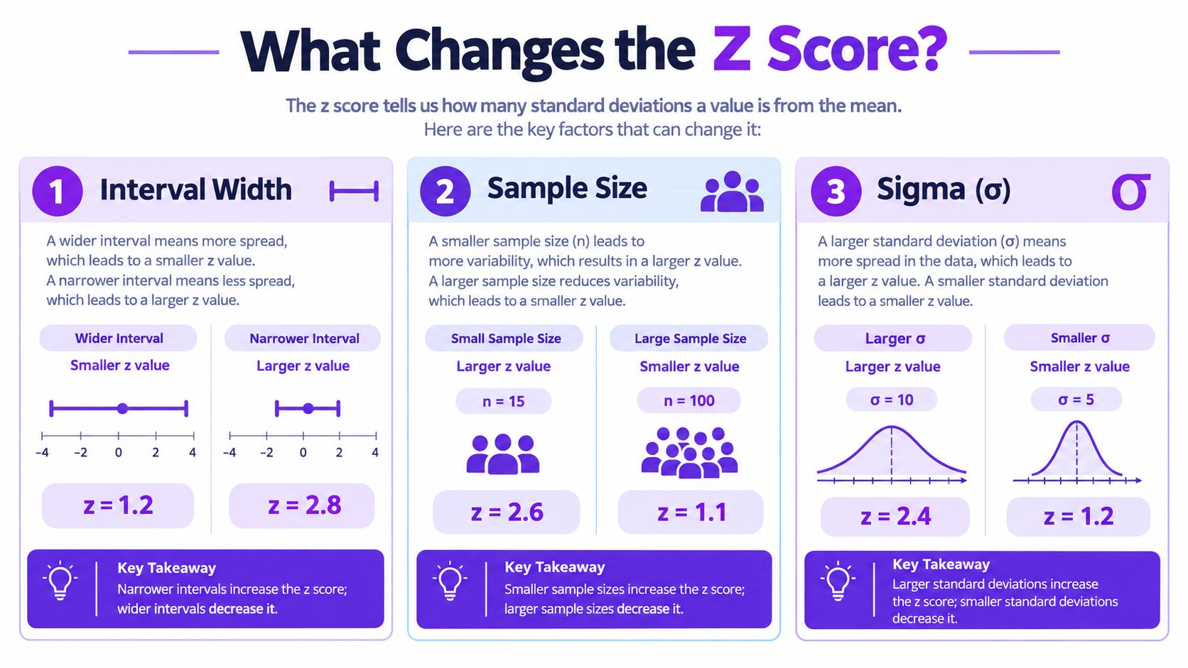
A useful way to read the formula is to ask what stayed fixed. If two estimates use the same confidence level and the same population variability, the estimate based on more observations will generally have a smaller standard error and a narrower interval. But when you are reverse-engineering an interval, don't infer the z score from sample size alone. Calculate it using the interval's half-width and the matching standard error.
The distinction between uncertainty in an estimate and a model's performance measures can matter in applied work. For a separate discussion of evaluation measures, see this guide to interpreting performance metrics.
When Z Stops Working and T Takes Over
The z calculation depends on a particular condition: the population standard deviation, (\sigma), is known. If you don't know it and substitute the sample standard deviation instead, you've introduced additional uncertainty. In that situation, the usual method for a confidence interval for a mean uses a t distribution, not a z distribution.
The t distribution resembles the standard normal distribution but has heavier tails. Those tails account for the extra uncertainty from estimating the population standard deviation using the sample. As the sample grows, the t distribution approaches the normal distribution, but choosing the right method still depends on the information and assumptions behind the analysis.
A practical first question is whether the report says the population standard deviation is known or whether it uses a sample-based estimate. If sigma is known and the interval was built using the normal model, the z formula applies. If sigma is unknown and estimated from the sample, use the t-based approach for the interval, with degrees of freedom determined by the method and sample design.
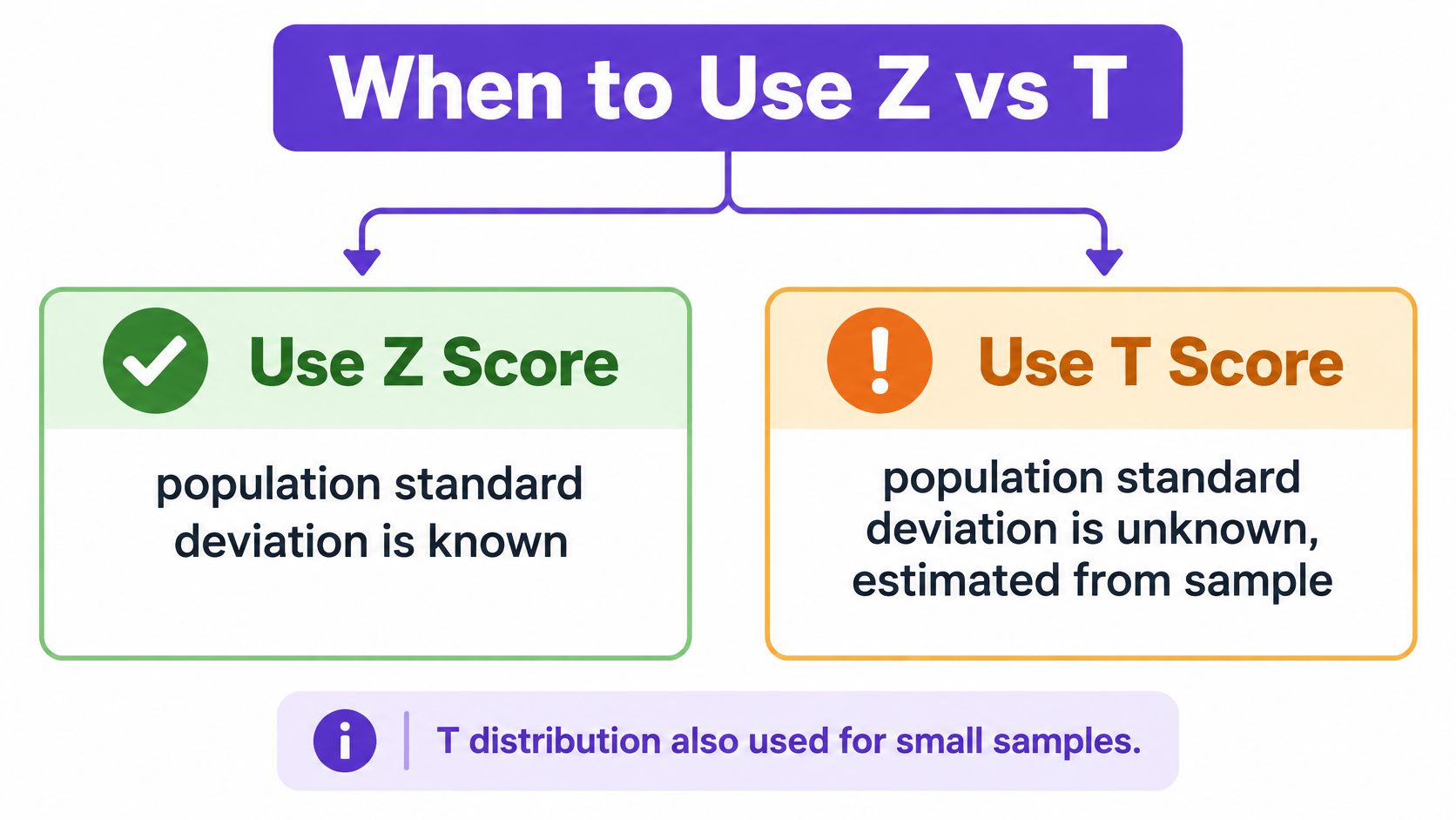
A small sample deserves particular care, especially when the data aren't reasonably modeled by the assumptions behind the interval. Don't assume that a z score becomes appropriate just because you can perform the algebra. If the original interval used a t critical value, dividing its margin of error by a standard error and labeling the result a z score won't recover the method's t multiplier.
Practical rule: Check how the interval was constructed before trying to identify its critical value. The formula's inputs and the method used to build the interval must match.
Putting the Conversion Together and Checking Your Work
To convert a confidence interval to a z score, divide its half-width by the standard error:
[ z = \frac{(U-L)/2}{\sigma/\sqrt{n}} ]
Here, (U) and (L) are the upper and lower endpoints. This calculation assumes a confidence interval for a mean using a known population standard deviation and the normal-distribution method.
Use this checklist when you're working from a report:
- Confirm the method. Check whether the interval is two-sided and whether it uses z or t.
- Record the endpoints. Label the upper and lower bounds clearly.
- Find the half-width. Subtract the lower bound from the upper bound and divide by two.
- Calculate the standard error. Use the appropriate standard deviation and sample size.
- Divide and compare. Divide the half-width by the standard error, then compare the result with the critical value implied by the reported confidence level.
The most useful check is whether the answer fits the method stated in the report. If a z-based interval claims a confidence level that doesn't match the calculated z, revisit the endpoints, the half-width, and the standard error. Make sure you haven't used the full interval width by mistake or treated an estimated standard deviation as known.
Once you can move from an interval to its critical value, you can reverse the process to build an interval from a z score. That foundation also helps with related tasks, such as interpreting a ROC curve. Practise the conversion with an interval whose inputs are clearly stated, and check each step against the method used to create it.
If you work with visual evidence as well as statistical results, AI Image Detector can analyze an image and provide a confidence score with an explanatory verdict. Try it with an image you need to verify, then compare its reasoning with the other evidence you have before drawing a conclusion.